kleemans.ch

The Natural Language Toolkit (NLTK) is a neat tool for analyzing, well, natural language in Python. It's my favorite tool for basic corpus analysis, and want to share some useful examples, based on the talking in the television show Scrubs.

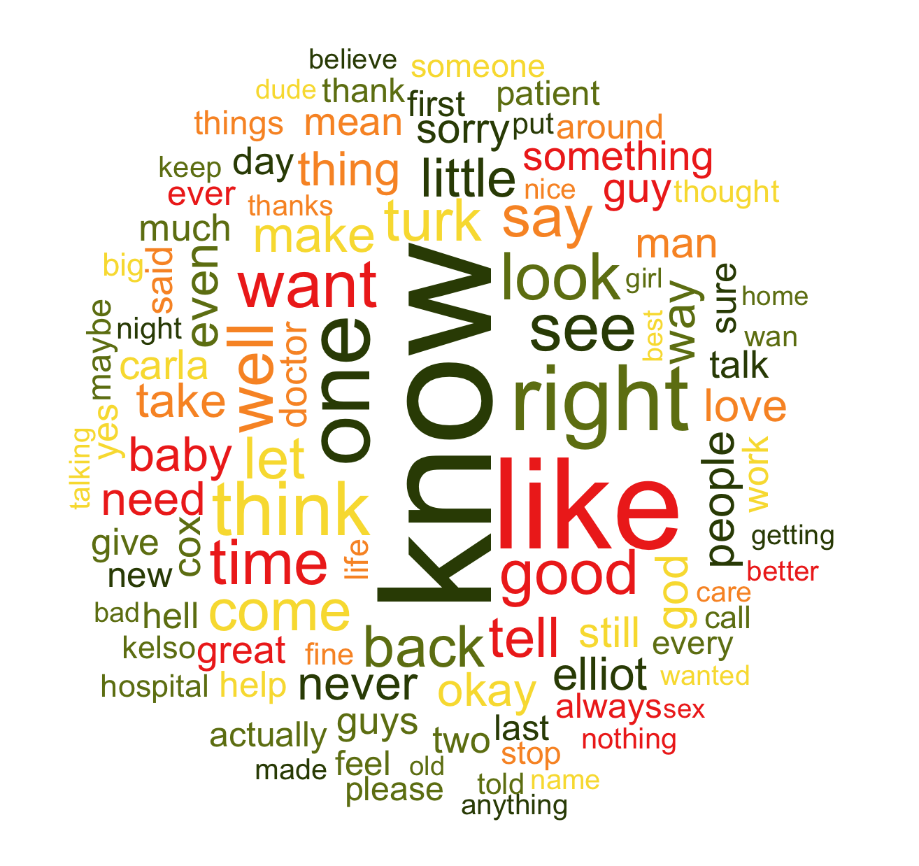
Word cloud of most used words in "Scrubs"

After cleaning up the text, we can generate the wordcloud above (see this earlier post on how to generate them).

Getting ready & gathering data

First of all, you'll need Python, which I assume you already have installed. To download NLTK via pip, just enter pip install nltk. After that, you'll be able to use the most basic functions, but for some cool extras you'll need to download some additional files. Using nltk.download(), you can download some corpus data (for example stopword dictionaries) and also some free available corpora, a popup will appear. For now, we'll use our own corpus, so you can just download the "book" part which covers a lot already.

Scrubs, which subtitles I will use as a base for the corpus, is a tv show about JD and his friends from med school on their way into their life as doctors in the hospital Sacred heart.

JD expressing his feelings towards Turk

I started rewatching it and thought it would be a nice corpus for doing some analysis on it, and thanks to all the busy Subscene all subtitles are available for download (here for example).

Subtitles in plain .srt or .sub Format look like this:

135
00:07:01,087 --> 00:07:04,579
Could you lend me a pen?
Quick as a porcupine's hiccup.

136
00:07:04,657 --> 00:07:07,524
# sexy jazz music #

137
00:07:09,796 --> 00:07:12,492
All right, there's only
one problem with this.

138
00:07:12,565 --> 00:07:14,590
(record scratches and music stops)

139
00:07:14,667 --> 00:07:16,828
OK, see ya, JD

140
00:07:17,570 --> 00:07:18,594
Kim, wait.

An incrementing number, the exact timespan and the text (sometimes with a simple markup) make up a single "screen" which will be shown for some seconds.

First of all extracted all text into a more handy format for later parsing, and after that followed a lot of cleaning up. Because there's no real standard for writing subtitles, sometimes actions, music, or even who speaks the line is included. I unified that into:

• music and songs are now indicated by # #
• actions are indicated by ( )
• due to sparse indication of who's speaking, I removed all speaker notations.
• removal of special characters, unification of ", `, '
• removal of additional text, attribution, ("Transcript by", "Subs by", "Special thanks to")

You can download the cleaned up subtitles here.

After that, I was able do gain some basic text metrics about the corpus:

• 182 episodes in 9 seasons
• 72'000 screens
• 2'870'000 characters of text

More stats to follow later. But first of all, we're loading the cleaned up subtitles into a NLTK corpus:

import nltk

with open('all_subtitles_clean.txt', 'r') as read_file:
    data = read_file.read()

data = data.decode("ascii", "ignore").encode("ascii")
tokens = nltk.word_tokenize(data)
text = nltk.Text(tokens)

Now we can work with the text as an object and use all the features NLTK provides.

Similarity and context

We can for example check what other similar words (used in similar context) exist for a given word:

>>> text.similar('surgeon')
doctor, guy, hospital, second, kid, man

Some other examples (shortened):

>>> text.similar('football')
outside baseball walking serving golf
>>> text.similar('freedom')
wrestle sleep prison smile kick coffee practice sunny break
>>> text.similar('vascular')
arterial heart surgical plastic pulmonary
>>> text.similar('relationship')
doctor guy baby time hospital girl patient problem life friend

That can yields some funny results, like freedom -> coffee. Note that for technical terms like vascular, the results like **arterial, heart, pulmonary*** are quite appropriate.

Another way to look at this is by directly comparing multiple words and show what similar contexts they share, regardless of their frequency.

For example the both main chief doctors, Dr. Cox and Dr. Kelso, often have similar patterns in which they are referred to:

>>> text.common_contexts(['Kelso', 'Cox'])
tell_that, what_said, because_has, dr_did, sorry_i, to_office

The results mean that the phrase shown exists often for both words, like:

• "tell Kelso that", "tell Cox that"
• "sorry Dr. Kelso I", "sorry Dr. Cox I"
• "to Kelso's office", "to Cox' office"

Note the "I ___ Dr. Cox" in the next example: He's the only one that appears in the same context as love and hate, so this suggests that strong feelings in both directions are directed towards him from the others.

>>> text.common_contexts(['love', 'hate'])
i_a, i_cox , i_your, i_about, you_that, ...

You can also look directly into the "surroundings" of a word, which is a popular method for classiscal text analysis:

>>> text.concordance('patient')
.. Could you drop an NG tube on the patient in 234 and then call the attending
n yesterday did n't really focus on patient care . The hospital does n't wan na
 a mistake , do n't admit it to the patient . Of course , if the patient is dec
to the patient . Of course , if the patient is deceased , and you 're sure , yo
ll me what to look for in a uraemic patient . Anyway , I 'm going for it . Infe
c insufficiency . That 's my girl . Patient number two . `` Superior mesenteric
 has to run the room , decides if a patient lives or dies . What , am I crazy ?
end to remember your names . If the patient has insurance , you treat them . If
 It 's a piece of cake . It 's your patient . You 're leaving ? That 's your pa
nt . You 're leaving ? That 's your patient , doctor . Good . That 's enough .
 She forgot to check the stats on a patient and gave me attitude . Did you tell
 new . Look , man . You 're a great patient . I like you enough to hope I never
se . That was a great catch on that patient with meningococcus . That actually
Severe swelling of the lips in this patient might be an indication of what ? An

You can modify how much will be shown left and right, and also how many lines should be shown (second argument):

>>> text.concordance('janitor', 40, lines=10)
Displaying 10 of 160 matches:
m a 37-year-old janitor . How d'you thi
ng with being a janitor . Really ? Than
. I 'll tell my janitor wife and all ou
ife and all our janitor kids that life
t . I think the janitor 's out to get m
 're cute . The janitor . This guy is a
the Holly Jolly Janitor . Little girl .
fixed . He 's a janitor . Yeah , but he
s . I 'm just a janitor . I do n't know
nothing but The Janitor . That 's not t

Frequency analysis

Now to some basic frequency analysis! The cool thing is that we can handle our text object just like a list, iterate over it, or get some basic attributes out of it:

>>> print len(text)
699901
>>> print len(set(text))
24583

That means the text consists of a total of nearly 700k words! On the second line, we first build a set out of our words (this will automatically remove all duplicates) and check the size: only 25k unique words!

We can now calculate the "lexical diversity" (unique words / total number of words), and see that the number of distinct words is just 3.5% of the total number of words! That's quite low compared to other texts (some corpora from NLTK have like 25%), and means that a lot repeats itself over and over.

We can also count specific words (or 'tokens') throughout the text:

>>> print text.count('bambi')
72
>>> print text.count('scrubs')
64

We can also define our own criteria and check for matching words, like extra long words:

>>> long_words = [w for w in text if len(w) > 25]
Whatever-the-hell-your-name-is
two-hours-after-his-shift-
Too-Scared-To-Get-ln-The-Game
Esophogeo-gastro-duodeno-colitis
bring-your-problems-to-work
Yesterday-l-Had-Chest-Hair
block-the-door-with-my-foot
Rin-Tin-Tin-Tin-Tin-Tin-Tin
you-leaving-the-room-whenever-I-enter-it
everandeverandeverandeveraneverandever
Aaaaaaaaaaaaaaagggggggggggggggggghhhhhhhhhhhhhhhhhhhh
aaagghhh-hagh-haaaaggghhhh
Noooooooooooooooooooooooooooooooooooooooooooooo
Riiiiiiiiiiiiiiiiiiiiiiiiiiiiiiiight
daaaaaaaiiiiiioooooooowwww
Buddy-buddy-buddy-buddy-buddy
What's-He-Over-Compensating-For
tickletickletickletickletickle
...

Another unit of text to look at are sentences. Also here NLTK has some predefined functions, so we don't have to look for . ! ? ourselves:

>>> print 'Number of sentences:', len(sents)
Number of sentences: 76821
>>> print 'Average char. length of sentence:', len(data)/len(sents)
Average char. length of sentence: 37.1235859986
>>> print 'Average nr. of words per sentence:', len(text)/len(sents)
Average nr. of words per sentence: 9.11080303563

Now for some frequency analysis per word, we're going to clean up the text some more: Decapitalize, removing punctuation marks, and remove stopwords. Stopwords are words which add no real value in text analysis, they appear in every text and are needed to get proper sentence structure, but they're not distinctive for most natural language analysis, so we're going to remove them.

# 1. de-capitalize
text_nostop = [w.lower() for w in text]

# 2. remove interpunctuation
interp = ['.', ',', '?', '!', ':', ';', '"', "'", ...]
text_nostop = [w for w in text_nostop if w not in interp]

# 3. remove stopwords
from nltk.corpus import stopwords
stopwords = stopwords.words('english')
my_stopwords = ["'s", "n't", '...', "'m", "'re", "'ll", ...]
with open('additional_stopwords.txt', 'r') as read_file:
    buckley_salton = read_file.read()
additional_stopwords = buckley_salton.split('\')

stopwords = stopwords + my_stopwords + additional_stopwords
text_nostop = [w for w in text_nostop if w not in stopwords]

fd_nostop = nltk.FreqDist(text_nostop) # new distribution

With our new distribution, we can

>>> for w, f in fd_nostop.most_common(100):
    print w + ':' + str(f)
hey:1418
time:1231
good:1216
turk:1126
back:1103
dr.:1087
make:914
baby:857
thing:846
elliot:808
god:803
people:801
love:796
man:732
guy:723
jd:711
carla:698
cox:650

We can also plot the most common words with their frequency:

>>> fd_nostop.plot(30, cumulative=False)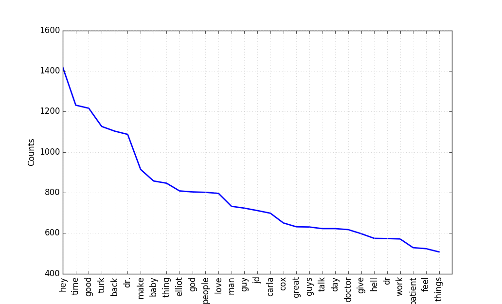

We can also get a summary of the most common collocations as seen before (a "quick glimpse what text is about"), only now the combinations are much more interesting because we filtered out all stopwords:

>>> text_nostop = nltk.Text(text_nostop)
text_nostop.collocations()
dr. cox; even though; last night; dr. kelso; sacred heart; dr. reid;
looks like; med school; high school; big deal; chief medicine; best
friend; feel like; little bit; mrs. wilk; every time; take care
dr. dorian; every day; john dorian; dr. turk; bob kelso; make
sure; last time; god sake; superman superman; number one; getting
married; bottom line; years ago; blah blah; med student; one thing;

It's about doctors, medicine, a hospital called Sacred Heart, John Dorian, his best friend, med school. Notice also common collocations like the "I'm no Superman" are listed here because they appear in each episode. Also phrases often used like Hey guys or blah blah and also "normal" word combinations like cell phone, bottom line, fair enough, leave alone and good morning appear.

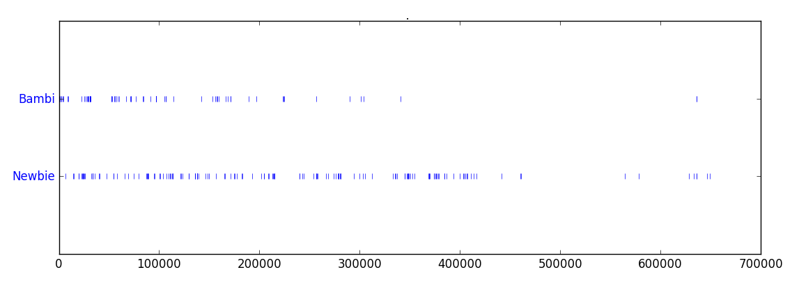
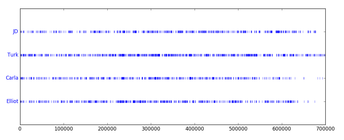
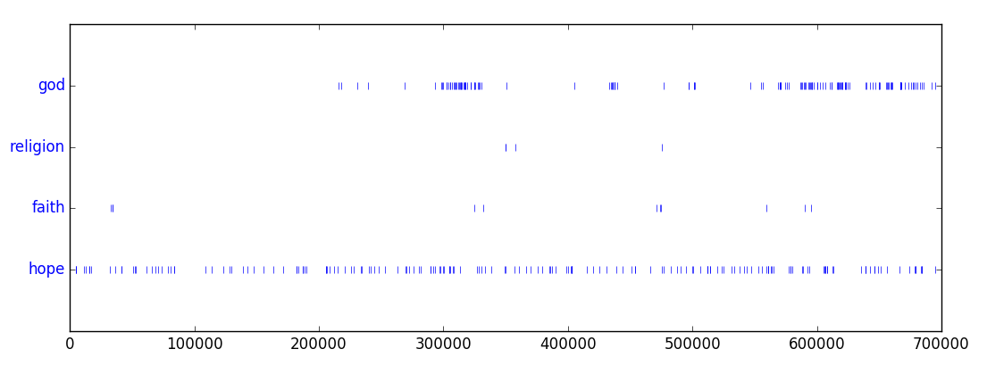
Dispersion plots

Another fun thing to do are dispersion plots. They show in which places of the text a certain word appears, marked by a small blue mark.

• Bambi vs Newbie: Dr. Cox' nickname sticks much longer than Carla's Bambi, both used to describe JD.

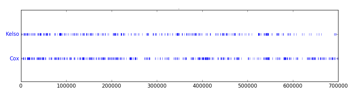
• Cox vs Kelso: Although both appear the whole time, we can spot differences regarding intensity and distribution. Cox appears more piled while Kelso seems more steady.

• The gang: In the beginning, most events are strictly observed based on JDs perspective (my guess why he's not appearing that much in the beginning), which seems to shift after some time, and he gets mentioned more. We can also see that Carla is not present in the latest season, and even before that her appearance is declining, in contrast to Elliot.

• hope, faith: Most words in this context are only used sporadically, only hope appears steadily throughout all the text.

Advanced use

After mastering the basics, there's lots more to discover, two quick examples here. Remember when we had kind of a summary with collocations? These are based on bigrams, words that are appearing together. We can find bi-, tri- and n-grams ourselves, let's look for the most appearing trigrams:

>>> trigrams = {}
>>> for trigram in nltk.trigrams(text):
...    if trigram in trigrams: trigrams[trigram] += 1
...    else: trigrams[trigram] = 1
... print '\'.join([' '.join(t) for t in trigrams if trigrams[t] > 400])
. It 's
. Oh ,
I ca n't
do n't know
. Well ,
I 'm gon
. You know
. You 're
. I do
I 'm not
? I 'm
. Yeah ,
I do n't
...

As expected, a lot of stopwords, but we see the most used "three word combinations" from the text. Remarkable is the use of "to know", which also is one of the most used words in general.

You can also analyze words by their usage in the sentence, NLTK has a built-in POS-Tagger which can tag each word with the (expected) usage in the sentence, as "part of speech":

>>> nltk.pos_tag(text[:18])
[('I', 'PRP'), ("'ve", 'VBP'), ('always', 'RB'), ('been', 'VBN'), 
('able', 'JJ'), ('to', 'TO'), ('sleep', 'VB'), ('through', 'IN'), 
('anything', 'NN'), ('.', '.'), ('Storms', 'NNP'), (',', ','), 
('sirens', 'VBZ'), (',', ','), ('you', 'PRP'), ('name', 'VBP'), 
('it', 'PRP'), ('.', '.')]

This would even allow us to draw some parsing trees for sentences, but for this we have to define our own grammar. Read here more words and their role in sentences, if you like.

I'm just going to construct a very simple grammar:

>>> mygrammar = nltk.CFG.fromstring("""
 S  -> NP VP
 Nom -> Adj Nom | N
 VP -> VP VP | VP PP | V Adj | V NP | V S | V NP PP
 PP -> Prep V | Prep Adj
 V    -> 'have' | 'been' | 'sleep'
 NP   -> 'I'
 Adj  -> 'always' | 'anything' | 'able'
 Prep -> 'to' | 'through'
 """)

Based on these production rules, like S -> NP VP (which means that a sentence S can be expanded to a noun phrase NP and a verbal phrase VP), NLTK will be able to figure out some possible tree structures. As always with natural language, there's tons of ambiguity to deal with, as a further reading I can recommend chapter 8 of the NLTK book.

We can now run the sentence together with our grammar through the parser, and it spits out possible sentence structures:

sentence = "I have always been able to sleep through anything".split(' ')
parser = nltk.ChartParser(mygrammar)
for tree in parser.parse(sentence):
  print(tree)

(S
  (NP I)
  (VP
    (VP (V have) (Adj always))
    (VP
      (VP (VP (V been) (Adj able)) (PP (Prep to) (V sleep)))
      (PP (Prep through) (Adj anything)))))
(S
  (NP I)
  (VP
    (VP
      (VP (VP (V have) (Adj always)) (VP (V been) (Adj able)))
      (PP (Prep to) (V sleep)))
    (PP (Prep through) (Adj anything))))
(S
  (NP I)
  (VP
    (VP
      (VP (V have) (Adj always))
      (VP (VP (V been) (Adj able)) (PP (Prep to) (V sleep))))
    (PP (Prep through) (Adj anything))))

Now that we have our grammar and a tree, we can print a parsed tree and even draw it:

>>> from nltk import Tree
from nltk.draw.util import CanvasFrame
from nltk.draw import TreeWidget

cf = CanvasFrame()
t = Tree.fromstring("(S (NP I) (VP (VP (V have) (Adj always)) (VP (VP (VP (V been) (Adj able)) (PP (Prep to) (V sleep))) (PP (Prep through) (Adj anything)))))")
tc = TreeWidget(cf.canvas(),t)
cf.add_widget(tc, 10, 10)

...which will generate the following tree structure.

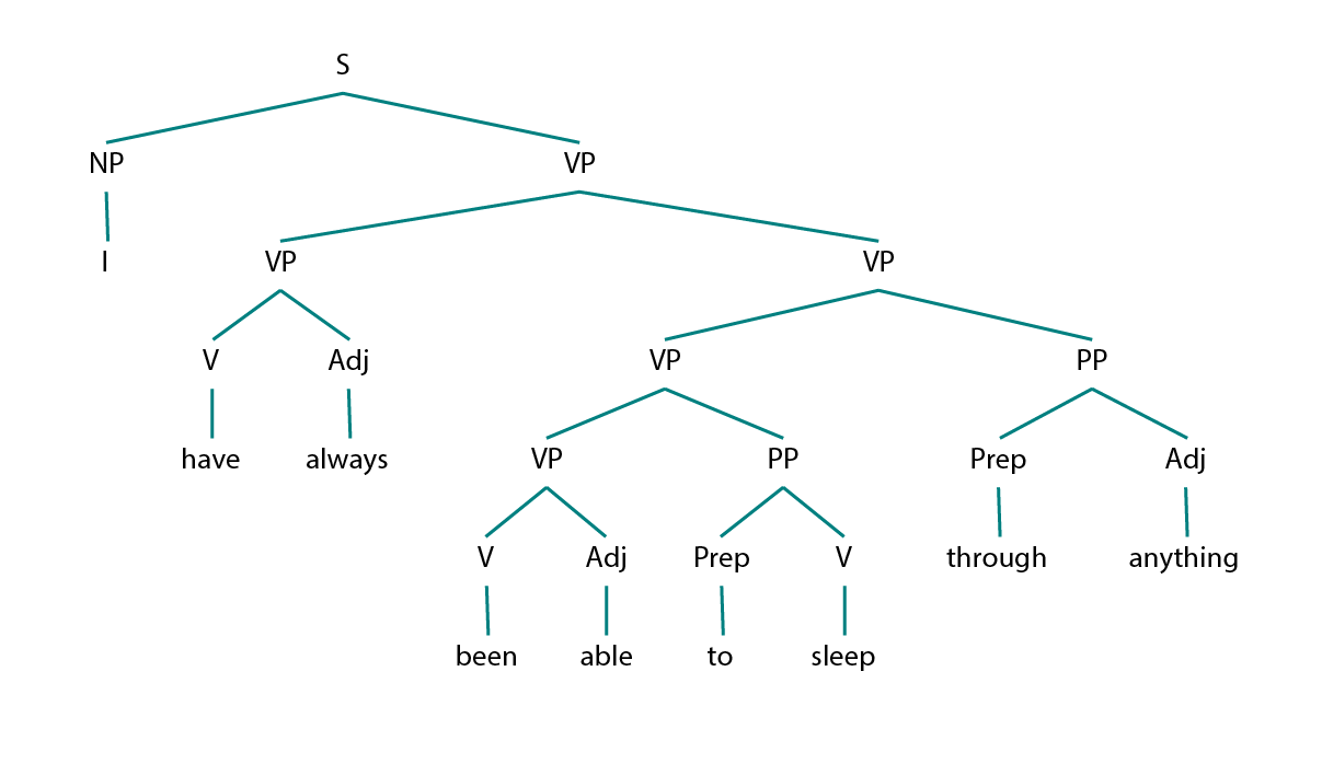
How cool is that?! :-)

Summary

NLTK is really simple and clean, and has tons of handy features out of the box, from frequency analysis, similarity and context analysis to dispersion plots, and even parsing and grammar trees.

All the examples are on Github, and also the base "corpus" of subtitles. I can also really recommend this cheat sheet and of course, the NLTK book.

Thanks for reading and happy parsing!