Statistics and Python
I'm a big fan of Python and grew fond of its SciPy libraries during a statistics class. It provides lots of statistical functions which I'd like to demonstrate in this post using specific examples. There's also a good overview of all functions at the SciPy docs.

For all the scripts to run you'll need to import SciPy and NumPy, and also pylab for the drawings:
import numpy as np
from scipy import stats
import pylab
Calculating basic sample data parameters
Given some sample data, you'll often want to find out some general parameters. This is most easily done with stats.describe:
data = [4, 3, 5, 6, 2, 7, 4, 5, 6, 4, 5, 9, 2, 3]
stats.describe(data)
>>> n=14, minmax=(2, 9), mean=4.643, variance=3.786,
skewness=0.589, kurtosis=-0.048
Here we immediately get some important parameters:
- n, the number of data points
- minimal and maximal values
- mean (average)
- variance, how far the data is spread out
- skewness and kurtosis, two measures of how the data "looks like"
To get the median, we'll use numpy:
np.median(data)
>>> 4.5
IQR (Interquartile range, range where 50% of the data lies):
np.percentile(data, 75) - np.percentile(data, 25)
>>> 2.5
MAD (Median absolute deviation):
np.median(np.absolute(data - np.median(data)))
>>> 1.5
Linear regression
Let's have a look at some similar looking, flat rectangles:

The numbers near each rectangle represent height, width and area. Suppose we want to find the correlation between two data sets, for example the width of the rectangles in respect to their area, we could look at that data:
One way to do this is linear regression. For linear regression, SciPy offers stats.linregress. With some sample data you can calculate the slope and y-interception:
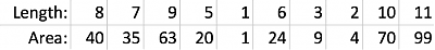
x = np.array([8, 7, 9, 5, 1, 6, 3, 2, 10, 11])
y = np.array([40, 35, 63, 20, 1, 24, 9, 4, 70, 99])
slope, intercept, r_val, p_val, std_err = stats.linregress(x, y)
print 'r value:', r_val
print 'y = ', slope, 'x + ', intercept
line = slope * x + intercept
pylab.plot(x, line, 'r-', x, y, 'o')
pylab.show()
The parameters for the function and also the Pearson coefficient are calculated:
>> y = 8.882x - 18.572
>> r value: 0.949
Combinatorics
Let's have a look at a some combinatorics functions.
For choosing 2 out of 20 items, there are 20*19 possible permutations (docs: scipy.special.perm).
For "from N choose k" we can use scipy.misc.comb. For example, if we have 20 elements and take 2 but don't consider the order (or regard them as set), this results in comb(20, 2).
from scipy.special import perm, comb
perm(20, 2)
>>> 380
comb(20, 2)
>>> 190
So the result would be 380 permutations or 190 unique combinations in total.
Fishers exact test
SciPy also has a lot of built in tests and methods where you can just plug in numbers and it will tell you the result.
One example is Fisher's exact test which can show some correlation between observations.
For example, if we have some medical data about people with hernia and some of them are truck drivers, we can check if those two "properties" are related:
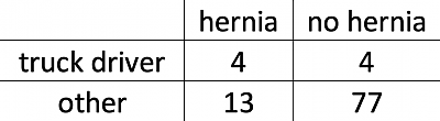
We can just enter the four main numbers (in the correct order) and get a result:
oddsratio, pvalue = scipy.stats.fisher_exact([[4, 4], [13, 77]])
>>> pvalue
0.0287822
The probability that we would observe this particular distribution of data is 2.88%, which is below 5%, so we may assume that our observations are significant and that (unfortunately) truck drivers are more likely to have a herniated disc.
Maybe some other time I'd like to show some more examples from SciPy with distributions and confidence intervals, but this as a introduction.
Also make sure to check out my blog post about Boxplots, which also use Python (with matplotlib to draw them).
Happy coding!
