Diagrams for logic in LaTeX

February 18, 2016

Looking through my school material, I found a lot of LateX graphics which I made for the according courses, and thought I'd share them.

Most of them use TikZ, an excellent graphics and drawing library for LaTeX. Some of the graphics here are modified examples from texample.net.

Beside some examples there is a short piece of code for demonstration purposes, at the bottom of the post there's a link for the full source code and also a compiled PDF with all the examples. It's quite some material and therefore a bit of a longer post :-) I grouped it into the following categories:

Binary trees
Logic circuits
Directed acyclic graphs (DAG)
Finite state machines (FSM)
Karnaugh maps
Ordered Binary Decision Diagrams (OBDD)
General graphs & functions
Misc

Binary trees

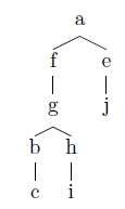
Drawing binary trees can bee a one-liner, using qtree:

\usepackage{qtree}
\Tree [.a [.f [.g [.b c ] [.h i ] ] ] [.e j ] ]

compiles to:

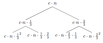
Another example (I believe it's from examining time complexity in loops):

Logic circuits

Especially with logic circuits the beauty of LaTeX became apparent when doing the exercises. Using the package signalflowdiagram (this one needs some additional files, see source) and the TikZ library shapes.gates.logic and shapes.gates.logic, it's possible to design your own logic circuits. It's still a lot of work

Decoder:

Half Adder:

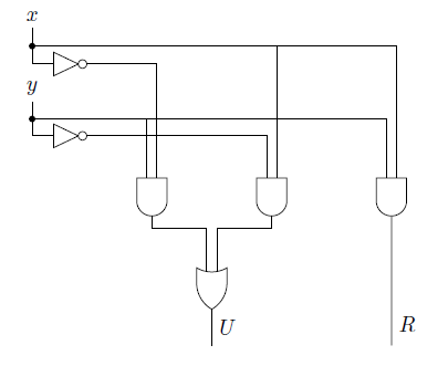
Some code for the half adder:

\tikzstyle{branch}=[fill,shape=circle,minimum size=3pt,inner sep=0pt]
\begin{tikzpicture}[label distance=2mm]
    % nodes
    \node (x) at (-1,6) {$x$};
    \node (y) at ($(x) + (0,-1.2)$) {$y$};
    \node[not gate US, draw] at ($(x)+(0.5,-0.8)$) (notx) {};
    \node[not gate US, draw] at ($(y)+(0.5,-0.8)$) (noty) {};
    \node[and gate US, draw, rotate=-90, logic gate inputs=nn] at (1,3) (A) {};
    \node[and gate US, draw, rotate=-90, logic gate inputs=nn] at ($(A)+(2,0)$) (B) {};
    \node[and gate US, draw, rotate=-90, logic gate inputs=nn] at ($(B)+(2,0)$) (C) {};
    \node[or gate US, draw, rotate=-90, logic gate inputs=nn] at ($(A)+(1,-1.5)$) (D) {};
    % draw NOT nodes
    \foreach \i in {x,y} {
        \path (\i) -- coordinate (punt\i) (\i |- not\i.input);
        \draw (\i) |- (punt\i) node[branch] {} |- (not\i.input);
    }
    % direct inputs
    \draw (puntx) -| (C.input 1);
    \draw (punty) -| (C.input 2);
    \draw (puntx) -| (B.input 1);
    \draw (punty) -| (A.input 2);
    \draw (notx) -| (A.input 1);
    \draw (noty) -| (B.input 2);
    \draw (A.output) -- ([yshift=-0.2cm]A.output) -| (D.input 2);
    \draw (B.output) -- ([yshift=-0.2cm]B.output) -| (D.input 1);
    \draw (C) -- ($(C) + (0, -1.8)$) -- node[right]{$R$} ($(C) + (0, -2.5)$);
    \draw (D.output) -- node[right]{$U$} ($(D) + (0, -1)$);
\end{tikzpicture}

Here I first draw the nodes based on the shapes.gates.logic-library shapes \ode[not gate US, draw] and then draw the inputs. Note that it's possible to affect how the lines are drawn by setting -| between the nodes.

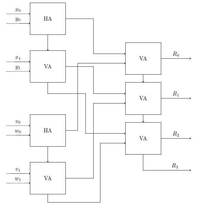
As you can see that's quite some code for a single graphic. For the adder network and half adder it's even worse :-), more complex circuits require a lot of tinkering with coordinates and shapes.

Adder network:

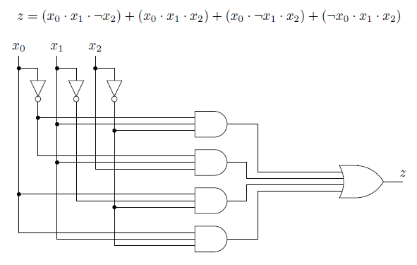
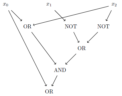
Logic circuit of a boolean function:

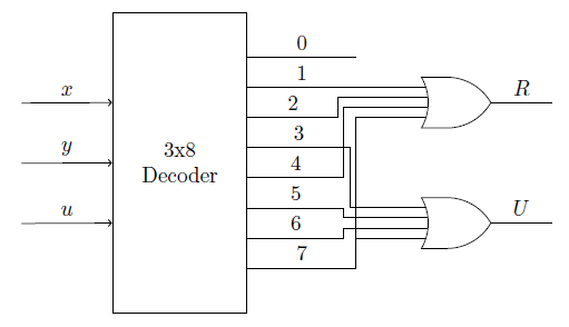
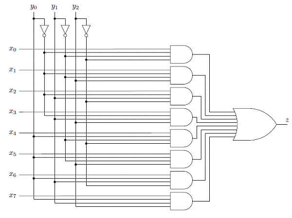
3-Mux Multiplexer:

Directed acyclic graphs (DAG)

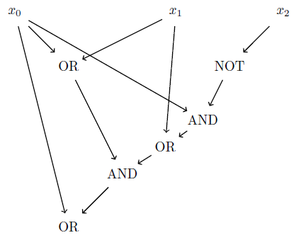
DAGs are quite easy to create. First you create the different nodes with name, displayed text and position:

\begin{center}
\begin{tikzpicture}[scale=1.4, auto,swap]
\foreach \pos/\name/\disp in {
  {(-2,4)/1/$x_0$}, 
  {(1,4)/2/$x_1$},
  {(3,4)/3/$x_2$}, 
  {(2,3)/4/NOT}, 
  {(1.5,2)/5/AND}, 
  {(.8,1.5)/6/OR}, 
  {(-1,3)/7/OR}, 
  {(0,1)/8/AND}, 
  {(-1,0)/9/OR}}
\node[minimum size=20pt,inner sep=0pt] (\name) at \pos {\disp};

Then you just connect them using \path and specify the type of line as an arrow (->):

\foreach \source/\dest in {
  1/5,1/7,1/9,
  2/6,2/7,
  3/4,
  4/5,
  5/6,
  6/8,
  7/8,
  8/9}
\path[draw,thick,->] (\source) -- node {} (\dest);
\end{tikzpicture}
\end{center}

Another example:

Finite state machines

Two graphics for Finite state machines. I already did something on this topic in an earlier blog post, check out my simulation for searching a path on a FSM.

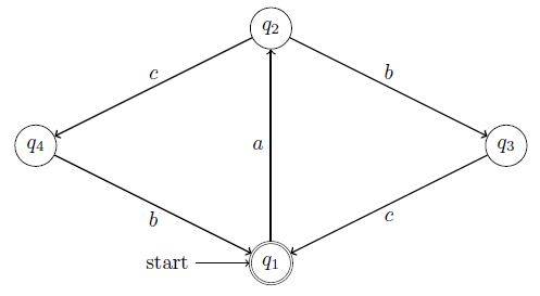
These can also be built with two loops, one for the nodes and the other one for the connections. Remember to use the TikZ library automata.

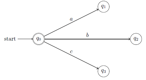
\usepackage{tikz}
\usetikzlibrary{automata}

\begin{tikzpicture}[scale=2, auto,swap]
\foreach \pos/\name/\disp/\initial/\accepting in {
  {(0,1)/q0/q_0/initial/accepting}, 
  {(2,0)/q3/q_3//},
  {(3,1)/q2/q_2//}, 
  {(2,2)/q1/q_1//}}
\node[state,\initial,\accepting,minimum size=20pt,inner sep=0pt] (\name) at \pos {$\disp$};
\foreach \source/\dest/\name/\pos in {
  q0/q1/a/above,
  q0/q2/b/above,
  q0/q3/c/above}
\path[draw,\pos,thick,->] (\source) -- node {$\name$} (\dest);
\end{tikzpicture}

Karnaugh maps

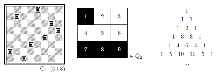
With Karnaugh maps, it is possible to simplify boolean algebra functions. For example, for boolean input variables A, B, C, D (which can either be true or false) and a function F(A, B, C, D) which maps them to a boolean output value you can draw the following Karnaugh map (for further reading, check the Quine-McCluskey algorithm, minterms and maxterms)

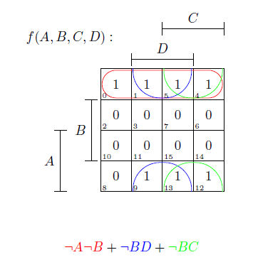
The diagram can be read as follows: For example at cell 3, B and D are overlapping = true, while A and C are false. So the function with the input F(0, 1, 0, 1) = 0.

Another Karnaugh diagram (can you figure out the function behind it? :-) ):

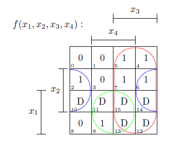
Karnaugh maps are really easy to draw with the kvmacro (which you have to include):

\input kvmacros.tex

\begin{center}
\karnaughmap{4}{$f(x_1,x_2,x_3,x_4):$}
{{$x_1$}{$x_3$}{$x_2$}{$x_4$}}{0010111101DDDDDD}
{
  \put(3,2){\color{red}\oval(1.9,3.9)}
  \put(4,2){\color{blue}\oval(1.9,1.9)[l]}
  \put(0,2){\color{blue}\oval(1.9,1.9)[r]}
  \put(2,1){\color{green}\oval(1.9,1.9)}
}
\end{center}

Ordered Binary Decision Diagrams (OBDD)

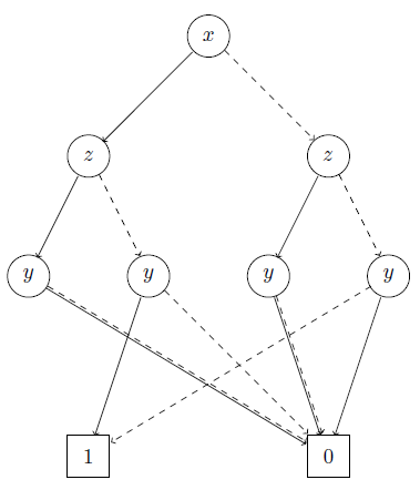
OBDDs are useful in debugging logic circuits (at least our professor told us so). They are drawn like the other graphs, defining the nodes (the end nodes as a special case with other looks) and in the last step linking them together with arrows.

A sample OBDD:

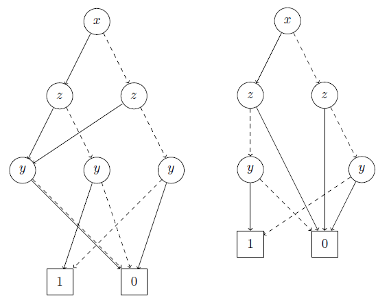
You can also do some operations on such a tree, which will reduce it an change its form (in german "Verjüngung" and "Elimination"). Also, the initial variable ordering is important and has an influence on how much you can optimize the tree.

Here is the equivalent graph in two more reduced forms:

General graphs & functions

Not strictly logic, but also functions, plotted with TikZ:

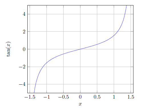
\begin{center}
\begin{tikzpicture}
  \begin{axis}[
  xlabel={$x$},
  xmin=-1.57, xmax=1.57,
  ymin=-5, ymax=5,
  ylabel={$\  an(x)$},
  domain=-2:2,
  samples=100,
  grid]
  \addplot+[no marks] function {tan(x)};
  \end{axis}
\end{tikzpicture}
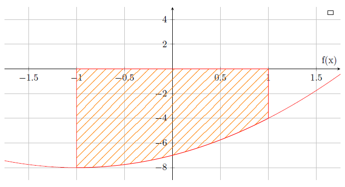
\end{center}

It's also possible to show the an integral area of a function:

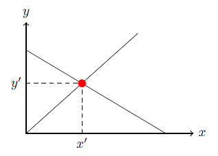
Two intersecting lines:

Two functions on a graph:

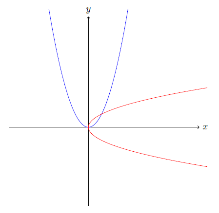
\begin{tikzpicture}
  \draw[->] (-3,0) -- (4.2,0) node[right] {$x$};
  \draw[->] (0,-3) -- (0,4.2) node[above] {$y$};
  \draw[scale=0.5,domain=-3:3,smooth,variable=\x,blue] 
        plot ({\x},{\x*\x});
  \draw[scale=0.5,domain=-3:3,smooth,variable=\y,red]  
        plot ({\y*\y},{\y});
\end{tikzpicture}

Misc

Bonus: Some more graphics which I dug up, also generated with LaTeX :-)

Downloads

You can download everything (and one or two more circuits which aren't listed here):

kleemans.ch

Static Pages

Search

Links